14 Mathematical appendix
This chapter contains remarks regarding the mathematical background of certain methods and concepts encountered in Chapters 7-11. Sections 14.2 and 14.3 consist of reworked materials from Thulin (2014b). Most of this chapter assumes some familiarity with mathematical statistics, on the level of Casella & Berger (2002) or Liero & Zwanzig (2012).
14.1 Bootstrap confidence intervals
We wish to construct a confidence interval for a parameter \(\theta\) based on a statistic \(t\). Let \(t_{obs}\) be the value of the statistic in the original sample, \(t_i^*\) be a bootstrap replicate of the statistic, for \(i=1,2,\ldots,B\), and \(t^*\) be the mean of the statistic among the bootstrap replicates. Let \(se^*\) be the standard error of the bootstrap estimate, and \(b^*=t^*-t_{obs}\) be the bias of the bootstrap estimate. For a confidence level \(1-\alpha\) (\(\alpha=0.05\) being a common choice), let \(z_{\alpha/2}\) be the \(1-\frac{\alpha}{2}\) quantile of the standard normal distribution (with \(z_{0.025}=1.9599\ldots\)). Moreover, let \(\theta_{\alpha/2}\) be the \(1-\frac{\alpha}{2}\)-quantile of the bootstrap distribution of the \(t_i^*\)’s.
The bootstrap normal confidence interval is
\[t_{obs}-b^*\pm z_{\alpha/2}\cdot se^*.\]
The bootstrap basic confidence interval is
\[\Big(2t_{obs}-\theta_{\alpha/2}, 2t_{obs}-\theta_{1-\alpha/2} \Big).\]
The bootstrap percentile confidence interval is
\[\Big(\theta_{1-\alpha/2}, \theta_{\alpha/2} \Big).\]
For the bootstrap BCa confidence interval, let
\[\hat{z}=\Theta^{-1}\Big(\frac{\#\{t_i^*<t_{obs}\}}{B}\Big),\]
where \(\Theta\) is the cumulative distribution function for the normal distribution. Let \(t_{(-i)}^*\) be the mean of the bootstrap replicates after deleting the \(i\):th replicate, and define the acceleration term
\[\hat{a}=\frac{\sum_{i=1}^n(t^*-t_{(-i)}^*)}{6\Big(\sum_{i=1}^n(t^*-t_{(-i)}^*)^2\Big)^{3/2}}.\]
Finally, let \[\alpha_1 = \Theta\Big(\hat{z}+\frac{\hat{z}+z_{1-\alpha/2}}{1-\hat{a}(\hat{z}+z_{1-\alpha/2})}\Big)\]
and
\[\alpha_2 = \Theta\Big(\hat{z}+\frac{\hat{z}+z_{\alpha/2}}{1-\hat{a}(\hat{z}+z_{\alpha/2})}\Big).\]
Then the confidence interval is
\[\Big(\theta_{\alpha_1}, \theta_{\alpha_2}\Big).\]
For the studentised bootstrap confidence interval, we additionally have an estimate \(se_t^*\) for the standard error of the statistic. Moreover, we compute \(q_i=\frac{t_i^*-t_{obs}}{se_t^*}\) for each bootstrap replicate, and define \(q_{\alpha/2}\) as the \(1-\frac{\alpha}{2}\)-quantile of the bootstrap distribution of \(q_i\)’s. The confidence interval is then
\[\Big(t_{obs}-se_t^*\cdot q_\alpha/2, t_{obs}+se_t^*\cdot q_{1-\alpha/2}\Big).\]
14.2 The equivalence between confidence intervals and hypothesis tests
Let \(\theta\) be an unknown parameter in the parameter space \(\Theta\subseteq\mathbb{R}\), and let the sample \(\mathbf{x}=(x_1,\ldots,x_n)\in\mathcal{X}^ n\subseteq\mathbb{R}^n\) be a realisation of the random variable \(\mathbf{X}=(X_1,\ldots,X_n)\). In frequentist statistics, there is a fundamental connection between interval estimation and point-null hypothesis testing of \(\theta\) , which we describe next. We define a confidence interval \(I_\alpha(\mathbf{X})\) as a random interval such that its coverage probability
\[\mbox{P}_\theta(\theta\in I_\alpha(\mathbf{X}))= 1-\alpha\qquad\mbox{for all }\alpha\in(0,1).\] Consider a two-sided test of the point-null hypothesis \(H_0(\theta_0): \theta=\theta_0\) against the alternative \(H_1(\theta_0): \theta\neq \theta_0\). Let \(\lambda(\theta_0,\mathbf{x})\) denote the p-value of the test. For any \(\alpha\in(0,1)\), \(H_0(\theta_0)\) is rejected at the level \(\alpha\) if \(\lambda(\theta_0,x)\leq\alpha\). The level \(\alpha\) rejection region is the set of \(\mathbf{x}\) which lead to the rejection of \(H_0(\theta_0)\):
\[ R_\alpha(\theta_0)=\{\mathbf{x}\in\mathbb{R}^n: \lambda(\theta_0,\mathbf{x})\leq\alpha\}.\]
Now, consider a family of two-sided tests with p-values \(\lambda(\theta,\mathbf{x})\), for \(\theta\in\Theta\). For such a family we can define an inverted rejection region
\[ Q_\alpha(\mathbf{x})=\{\theta\in\Theta: \lambda(\theta,\mathbf{x})\leq\alpha\}.\]
For any fixed \(\theta_0\), \(H_0(\theta_0)\) is rejected if \(\mathbf{x}\in R_\alpha(\theta_0)\), which happens if and only if \(\theta_0\in Q_\alpha(\mathbf{x})\), that is,
\[ \mathbf{x}\in R_\alpha(\theta_0) \Leftrightarrow \theta_0\in Q_\alpha(\mathbf{x}). \] If the test is based on a test statistic with a completely specified absolutely continuous null distribution, then \(\lambda(\theta_0,\mathbf{X})\sim \mbox{U}(0,1)\) under \(H_0(\theta_0)\) (Liero & Zwanzig, 2012). Then
\[ \mbox{P}_{\theta_0}(\mathbf{X}\in R_\alpha(\theta_0))=\mbox{P}_{\theta_0}(\lambda(\theta_0,\mathbf{X})\leq\alpha)=\alpha. \] Since this holds for any \(\theta_0\in\Theta\) and since the equivalence relation \(\mathbf{x}\in R_\alpha(\theta_0) \Leftrightarrow \theta_0\in Q_\alpha(\mathbf{x})\) implies that
\[\mbox{P}_{\theta_0}(\mathbf{X}\in R_\alpha(\theta_0))=\mbox{P}_{\theta_0}(\theta_0\in Q_\alpha(\mathbf{X})),\]
it follows that the random set \(Q_\alpha(\mathbf{x})\) always covers the true parameter \(\theta_0\) with probability \(\alpha\). Consequently, letting \(Q_\alpha^C(\mathbf{x})\) denote the complement of \(Q_\alpha(\mathbf{x})\), for all \(\theta_0\in\Theta\) we have
\[\mbox{P}_{\theta_0}(\theta_0\in Q_\alpha^C(\mathbf{X}))=1-\alpha,\] meaning that the complement of the inverted rejection region is a \(1-\alpha\) confidence interval for \(\theta\). This equivalence between a family of tests and a confidence interval \(I_\alpha(\mathbf{x})=Q_\alpha^C(\mathbf{x})\), illustrated in Figure 14.1, provides a simple way of constructing confidence intervals through test inversion, and vice versa.
The figure shows the rejection regions and confidence intervals corresponding to the \(z\)-test for a normal mean, for different null means \(\theta\) and different sample means \(\bar{x}\), with \(\sigma=1\). \(H_0(\theta)\) is rejected if \((\bar{x},\theta)\) is in the shaded light grey region. Shown in dark grey is the rejection region \(R_{0.05}(-0.9)=(-\infty,-1.52)\cup(-0.281,\infty)\) and the confidence interval \(I_{0.05}(1/2)=Q_{0.05}^C(1/2)=(-0.120,1.120)\).
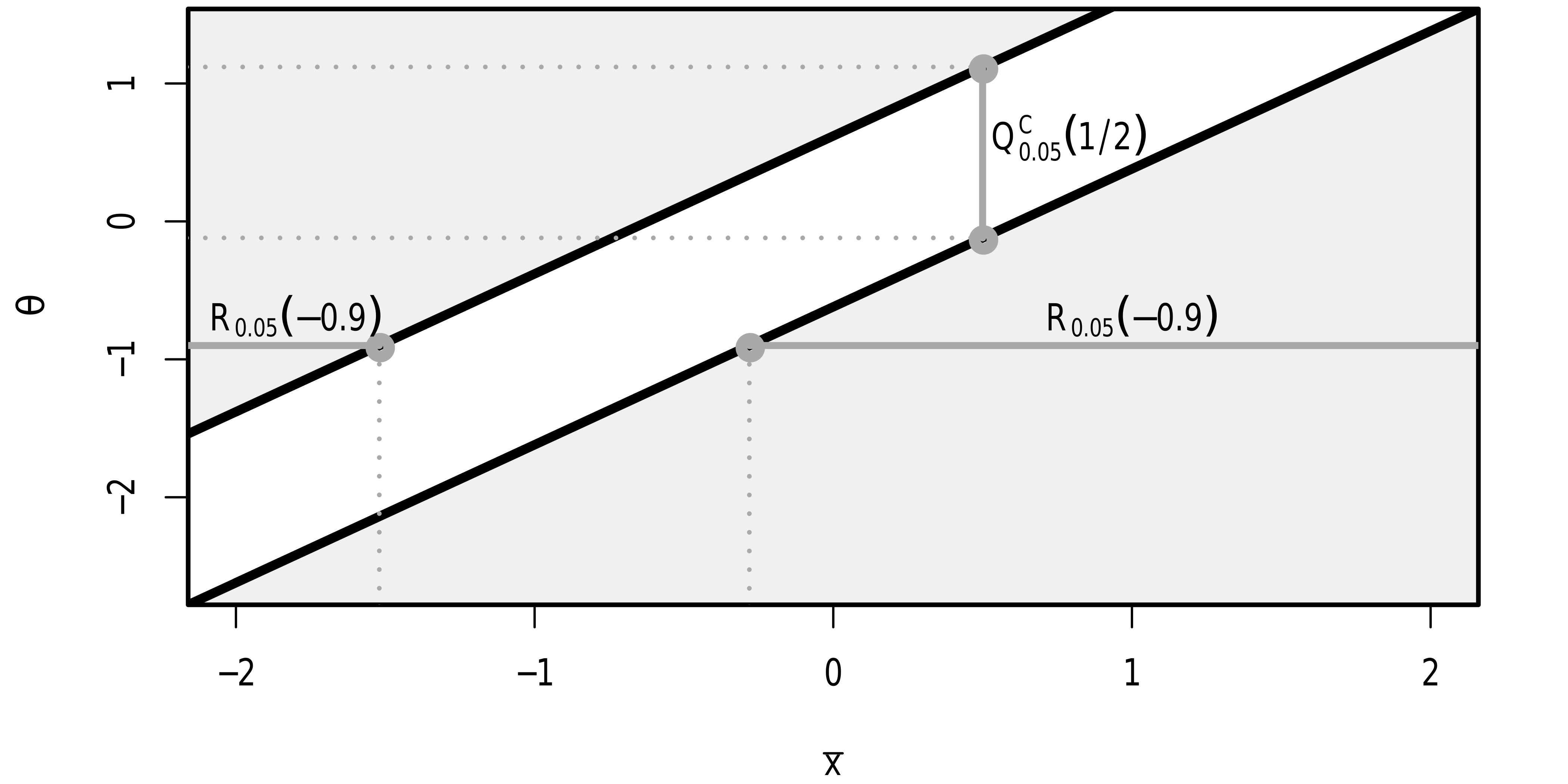
Figure 14.1: Equivalence between confidence intervals and hypothesis tests.
14.3 Two types of p-values
The symmetric argument in perm.t.test and boot.t.test controls how the p-values of the test are computed. In most cases, the difference is not that large:
library(MKinfer)
library(ggplot2)
boot.t.test(sleep_total ~ vore, data =
              subset(msleep, vore == "carni" | vore == "herbi"),
            symmetric = FALSE)

boot.t.test(sleep_total ~ vore, data =
              subset(msleep, vore == "carni" | vore == "herbi"),
            symmetric = TRUE)
In other cases, the choice matters more. Below, we will discuss the difference between the two approaches.
Let \(T(\mathbf{X})\) be a test statistic on which a two-sided test of the point-null hypothesis that \(\theta=\theta_0\) is based, and let \(\lambda(\theta_0,\mathbf{x})\) denote its p-value. Assume for simplicity that \(T(\mathbf{x})<0\) implies that \(\theta<\theta_0\) and that \(T(\mathbf{x})>0\) implies that \(\theta>\theta_0\). We’ll call the symmetric = FALSE scenario the twice-the-smaller-tail approach to computing p-values. In it, the first step is to check whether \(T(\mathbf{x})<0\) or \(T(\mathbf{x})>0\). “At least as extreme as the observed” is in a sense redefined as “at least as extreme as the observed, in the observed direction”. If the median of the null distribution of \(T(\mathbf{X})\) is 0, then, for \(T(\mathbf{x})>0\),
\[ \mbox{P}_{\theta_0}(T(\mathbf{X})\geq T(\mathbf{x})|T(\mathbf{x})>0)=2\cdot\mbox{P}_{\theta_0}(T(\mathbf{X})\geq T(\mathbf{x})),\] i.e., twice the unconditional probability that \(T(\mathbf{X})\geq T(\mathbf{x})\). Similarly, for \(T(\mathbf{x})<0\),
\[ \mbox{P}_{\theta_0}(T(\mathbf{X})\leq T(\mathbf{x})|T(\mathbf{x})<0)=~2\cdot\mbox{P}_{\theta_0}(T(\mathbf{X})\leq T(\mathbf{x})).\] Moreover,
\[ \mbox{P}_{\theta_0}(T(\mathbf{X})\geq T(\mathbf{x}))<\mbox{P}_{\theta_0}(T(\mathbf{X})\leq T(\mathbf{x}))\qquad\mbox{when}\qquad T(\mathbf{x})>0\] and
\[ \mbox{P}_{\theta_0}(T(\mathbf{X})\geq T(\mathbf{x}))>\mbox{P}_{\theta_0}(T(\mathbf{X})\leq T(\mathbf{x}))\qquad\mbox{when}\qquad T(\mathbf{x})<0.\] Consequently, the p-value using this approach can in general be written as
\[ \lambda_{TST}(\theta_0,\mathbf{x}):=\min\Big(1,~~2\cdot\mbox{P}_{\theta_0}(T(\mathbf{X})\geq T(\mathbf{x})),~~2\cdot\mbox{P}_{\theta_0}(T(\mathbf{X})\leq T(\mathbf{x}))\Big).\]
This definition of the p-value is frequently used also in situations where the median of the null distribution of \(T(\mathbf{X})\) is not 0, despite the fact that the interpretation of the p-value as being conditioned on whether \(T(\mathbf{x})<0\) or \(T(\mathbf{x})>0\) is lost.
At the level \(\alpha\), if \(T(\mathbf{x})>0\) the test rejects the hypothesis \(\theta=\theta_0\) if
\[ \lambda_{TST}(\theta_0,\mathbf{x})=\min\Big(1,2\cdot\mbox{P}_{\theta_0}(T(\mathbf{X})\geq T(\mathbf{x}))\Big)\leq\alpha.\]
This happens if and only if the one-sided test of \(\theta\leq \theta_0\), also based on \(T(\mathbf{X})\), rejects its null hypothesis at the \(\alpha/2\) level. By the same reasoning, it is seen that the rejection region of a level \(\alpha\) twice-the-smaller-tail test always is the union of the rejection regions of two level \(\alpha/2\) one-sided tests of \(\theta\leq \theta_0\) and \(\theta\geq \theta_0\), respectively. The test puts equal weight to the two types of type I errors: false rejection in the two different directions. The corresponding confidence interval is therefore also equal-tailed, in the sense that the non-coverage probability is \(\alpha/2\) on both sides of the interval.
Twice-the-smaller-tail p-values are in a sense computed by looking only at one tail of the null distribution. In the alternative approach, symmetric = TRUE, we use strictly two-sided p-values. Such a p-value is computed using both tails, as follows:
\(\lambda_{STT}(\theta_0,\mathbf{x})=\mbox{P}_{\theta_0}\Big(|T(\mathbf{X})|\geq |T(\mathbf{x})|\Big)=\mbox{P}_{\theta_0}\Big(\{\mathbf{X}: T(\mathbf{X})\leq -|T(\mathbf{x})|\}\cup\{\mathbf{X}: T(\mathbf{X})\geq |T(\mathbf{x})|\}\Big).\)
Under this approach, the directional type I error rates will in general not be equal to \(\alpha/2\), so that the test might be more prone to falsely reject \(H_0(\theta_0)\) in one direction than in another. On the other hand, the rejection region of a strictly two-sided test is typically smaller than its twice-the-smaller-tail counterpart. The coverage probabilities of the corresponding confidence interval \(I_\alpha(\mathbf{X})=(L_\alpha(\mathbf{X}),U_\alpha(\mathbf{X}))\) therefore satisfies the condition that
\[\mbox{P}_\theta(\theta\in I_\alpha(\mathbf{X}))= 1-\alpha\qquad\mbox{for all }\alpha\in(0,1),\]
but not the stronger condition
\[ \mbox{P}_\theta(\theta<L_\alpha(\mathbf{X}))=\mbox{P}_\theta(\theta>U_\alpha(\mathbf{X}))=\alpha/2\qquad\mbox{for all } \alpha\in(0,1).\]
For parameters of discrete distributions, strictly two-sided hypothesis tests and confidence intervals can behave very erratically (Thulin & Zwanzig, 2017). Twice-the-smaller-tail methods are therefore always preferable when working with count data.
It is also worth noting that if the null distribution of \(T(\mathbf{X})\) is symmetric about 0,
\[\mbox{P}_{\theta_0}(T(\mathbf{X})\geq T(\mathbf{x}))=\mbox{P}_{\theta_0}(T(\mathbf{X})\leq -T(\mathbf{x})).\]
For \(T(\mathbf{x})>0\), unless \(T(\mathbf{X})\) has a discrete distribution,
\[\begin{split} \lambda_{TST}(\theta_0,\mathbf{x})&=2\cdot \mbox{P}_{\theta_0}(T(\mathbf{X})\geq T(\mathbf{x}))\\&=\mbox{P}_{\theta_0}(T(\mathbf{X})\geq T(\mathbf{x}))+\mbox{P}_{\theta_0}(T(\mathbf{X})\leq -T(\mathbf{x}))=\lambda_{STT}(\theta_0,\mathbf{x}), \end{split}\]
meaning that the twice-the-smaller-tail and strictly two-sided approaches coincide in this case. The ambiguity related to the definition of two-sided p-values therefore only arises under asymmetric null distributions.
14.4 Deviance tests
Consider a model with \(p=n\), having a separate parameter for each observation. This model will have a perfect fit, and among all models, it attains the maximum achievable likelihood. It is known as the saturated model. Despite having a perfect fit, it is useless for prediction, interpretation and causality, as it is severely overfitted. It is however useful as a baseline for comparison with other models, i.e., for checking goodness-of-fit: our goal is to find a reasonable and useful model with almost as good a fit.
Let \(L(\hat{\mu},y)\) denote the log-likelihood corresponding to the ML-estimate for a model, with estimates \(\hat{\theta}_i\). Let \(L(y,y)\) denote the log-likelihood for the saturated model, with estimates \(\tilde{\theta}_i\). For an exponential dispersion family, i.e., a distribution of the form
\[f(y_i; \theta_i,\phi)=\exp\Big(\lbrack y_i\theta_i-b(\theta_i)\rbrack/a(\phi)+c(y_i,\phi)\Big),\]
(the binomial and Poisson distributions being examples of this), we have
\[L(y,y)-L(\hat{\mu},y)=\sum_{i=1}^n(y_i\tilde{\theta}_i-b(\tilde{\theta}_i))/a(\phi)-\sum_{i=1}^n(y_i\hat{\theta}_i-b(\hat{\theta}_i))/a(\phi).\]
Typically, \(a(\phi)=\phi/\omega_i\), in which case this becomes
\[\sum_{i=1}^n\omega_i\Big(y_i(\tilde{\theta}_i-\hat{\theta}_i)-b(\tilde{\theta}_i)+b(\hat{\theta}_i)\Big)/\phi=:\frac{D(y,\hat{\mu})}{2\phi},\]
where the statistic \(D(y,\hat{\mu})\) is called the deviance.
The deviance is essentially the difference between the log-likelihoods of a model and of the saturated model. The greater the deviance, the poorer the fit. It holds that \(D(y,\hat{\mu})\geq 0\), with \(D(y,\hat{\mu})=0\) corresponding to a perfect fit.
Deviance is used to test whether two models are equal. Assume that we have two models:
- \(M_0\), which has \(p_0\) parameters, with fitted values \(\hat{\mu}_0\),
- \(M_1\), which has \(p_1>p_0\) parameters, with fitted values \(\hat{\mu}_1\).
We say that the models are nested, because \(M_0\) is a special case of \(M_1\), corresponding to some of the \(p_1\) parameters of \(M_1\) being 0. If both models give a good fit, we prefer \(M_0\) because of its (relative) simplicity. We have \(D(y,\hat{\mu}_1)\leq D(y,\hat{\mu}_0)\), since simpler models have larger deviances. Assuming that \(M_1\) holds, we can test whether \(M_0\) holds by using the likelihood ratio-test statistic \(D(y,\hat{\mu}_0)-D(y,\hat{\mu}_1).\) If we reject the null hypothesis, \(M_0\) fits the data poorly compared to \(M_1\). Otherwise, the fit of \(M_1\) is not significantly better and we prefer \(M_0\) because of its simplicity.
14.5 Regularised regression
Linear regression is a special case of generalised linear regression. Under the assumption of normality, the least squares estimator is the maximum likelihood estimator in this setting. In what follows, we will therefore discuss how the maximum likelihood estimator is modified when using regularisation, bearing in mind that this also includes the ordinary least squares estimator for linear models.
In a regularised GLM, it is not the likelihood \(L(\beta)\) that is maximised, but a regularised function \(L(\beta)\cdot p(\lambda,\beta)\), where \(p\) is a penalty function that typically forces the resulting estimates to be closer to 0, which leads to a stable solution. The shrinkage parameter \(\lambda\) controls the size of the penalty, and therefore how much the estimates are shrunk toward 0. When \(\lambda=0\), we are back at the standard maximum likelihood estimate.
The most popular penalty terms correspond to common \(L_q\)-norms. On a log-scale, the function to be maximised is then
\[\ell(\beta)+\lambda\sum_{i=1}^p|\beta_i|^q,\]
where \(\ell(\beta)\) is the loglikelihood of \(\beta\) and \(\sum_{i=1}^p|\beta_i|^q\) is the \(L_q\)-norm, with \(q\geq 0\). This is equivalent to maximising \(\ell(\beta)\) under the constraint that \(\sum_{i=1}^p|\beta_i|^q\leq\frac{1}{h(\lambda)}\), for some increasing positive function \(h\).
In Bayesian estimation, a prior distribution \(p(\beta)\) for the parameters \(\beta_i\) is used. The estimates are then computed from the conditional distribution of the \(\beta_i\) given the data, called the posterior distribution. Using Bayes’ theorem, we find that
\[P(\beta|\mathbf{x})\propto L(\beta)\cdot p(\beta),\]
i.e., that the posterior distribution is proportional to the likelihood times the prior. The Bayesian maximum a posteriori estimator (MAP) is found by maximising the above expression (i.e., finding the mode of the posterior). This is equivalent to the estimates from a regularised frequentist model with penalty function \(p(\beta)\), meaning that regularised regression can be motivated both from a frequentist and a Bayesian perspective.
When the \(L_2\) penalty is used, the regularised model is called ridge regression, for which we maximise
\[\ell(\beta)+\lambda\sum_{i=1}^p\beta_i^2.\]
In a Bayesian context, this corresponds to putting a standard normal prior on the \(\beta_i\). This method has been invented and reinvented by several authors, from the 1940s onwards, among them Hoerl & Kennard (1970). The \(\beta_i\) can become very small but are never pushed all the way down to 0. The name comes from the fact that in a linear model, the OLS estimate is \(\hat{\beta}=(\mathbf{X}^T\mathbf{X})^{-1}\mathbf{X}^T\mathbf{y}\), whereas the ridge estimate is \(\hat{\beta}=(\mathbf{X}^T\mathbf{X}+\lambda \mathbf{I})^{-1}\mathbf{X}^T\mathbf{y}\). The \(\lambda \mathbf{I}\) is the “ridge”.
When the \(L_1\) penalty is used, the regularised model is called the lasso (Least Absolute Shrinkage and Selection Operator), for which we maximise
\[\ell(\beta)+\lambda\sum_{i=1}^p|\beta_i|.\]
In a Bayesian context, this corresponds to putting a standard Laplace prior on the \(\beta_i\). For this penalty, as \(\lambda\) increases, more and more \(\beta_i\) become 0, meaning that we can simultaneously perform estimation and variable selection!