10 Structural equation models, factor analysis, and mediation
Factor analysis and structural equation models let us model abstract nonmeasurable concepts, like intelligence and quality of life, called latent variables. These models have a rich theoretical framework which also allows us to extend regression models to include mediators that help explain causal pathways.
After reading this chapter, you will be able to use R to:
- Use exploratory factor analysis to find latent variables in your data,
- Use confirmatory factor analysis to test hypotheses related to latent variables,
- Fit structural analysis to your models, and
- Run mediation analyses to find mediated and moderated effects in regression models.
10.1 Exploratory factor analysis
The purpose of factor analysis is to describe and understand the correlation structure for a set of observable variables through a smaller number of unobservable underlying variables, called factors or latent variables. These are thought to explain the values of the observed variables in a causal manner. Latent variables can represent measurable but unobserved variables, but more commonly represent abstract concepts such as wisdom or quality of life.
Factor analysis is a popular tool in psychometrics. Among other things, it is used to identify latent variables that explain people’s results on different tests, e.g., related to personality, intelligence, or attitude.
10.1.1 Running a factor analysis
We’ll use the psych package, along with the associated package GPArotation, for our analyses. Let’s install them:
For our first example of factor analysis, we’ll be using the attitude data that comes with R. It describes the outcome of a survey of employees at a financial organisation. Have a look at its documentation to read about the variables in the dataset:
To fit a factor analysis model to these data, we can use fa from psych. fa requires us to specify the number of factors used in the model. We’ll get back to how to choose the number of factors, but for now, let’s go with 2:
library(psych)
# Fit factor model:
attitude_fa <- fa(attitude, nfactors = 2,
                  rotate = "oblimin", fm = "ml")
fa does two things for us. First, it fits a factor model to the data, which yields a table of factor loadings, i.e., the correlation between the two unobserved factors and the observed variables. However, there is an infinite number of mathematically valid factor models for any given dataset. Therefore, the factors are rotated according to some rule to obtain a factor model that hopefully allows for easy and useful interpretation. Several methods can be used to fit the factor model (set using the fm argument in fa) and for rotation of the solution (set using rotate). We’ll look at some of the options shortly.
Before that, we’ll print the result, showing the factor loadings (after rotation). We’ll also plot the resulting model using fa.diagram, showing the correlation between the factors and the observed variables:
The first factor is correlated to the variables advance, learning, and raises. We can perhaps interpret this factor as measuring the employees’ career opportunity at the organisation. The second factor is strongly correlated to complaints and (overall) rating, but also to a lesser degree correlated to raises, learning, and privileges. This maybe can be interpreted as measuring how the employees feel they are treated at the organisation.
We can also see that the two factors are correlated. In some cases, it makes sense to expect the factors to be uncorrelated. In that case, we can change the rotation method used, from oblimin (which yields oblique rotations, allowing for correlations - usually a good default) to varimax, which yields uncorrelated factors:
attitude_fa <- fa(attitude, nfactors = 2,
                  rotate = "varimax", fm = "ml")
fa.diagram(attitude_fa, simple = FALSE)
In this case, the results are fairly similar.
The fm = "ml" setting means that maximum likelihood estimation of the factor model is performed, under the assumption of a normal distribution for the data. Maximum likelihood estimation is widely recommended for estimation of factor models, and it can often work well even for non-normal data (Costello & Osborne, 2005). However, there are cases where it fails to find useful factors. fa offers several different estimation methods. A good alternative is minres, which often works well when maximum likelihood fails:
attitude_fa <- fa(attitude, nfactors = 2,
                  rotate = "oblimin", fm = "minres")
fa.diagram(attitude_fa, simple = FALSE)
Once again, the results are similar to what we saw before. In other examples, the results differ more. When choosing which estimation method and rotation to use, bear in mind that in an exploratory study, there is no harm in playing around with a few different methods. After all, your purpose is to generate hypotheses rather than confirm them, and looking at the data in a few different ways will help you do that (we’ll discuss how to test hypotheses related to factors in Section 10.2).
10.1.2 Choosing the number of factors
To determine the number of factors that are appropriate for a particular dataset, we can draw a scree plot with scree. This is interpreted in the same way as for principal components analysis (Section 4.11) and centroid-based clustering (Section 4.12.3) – we look for an “elbow” in the plot, which tells us at which point adding more factors no longer contributes much to the model:
A useful alternative version of this is provided by fa.parallel, which adds lines showing what the scree plot would look like for randomly generated uncorrelated data of the same size as the original dataset. As long as the blue line, representing the actual data, is higher than the red line, representing randomly generated data, adding more factors improves the model:
Some older texts recommend that only factors with an eigenvalue (the y-axis in the scree plot) greater than 1 be kept in the model. It is widely agreed that this so-called Kaiser rule is inappropriate (Costello & Osborne, 2005), as it runs the risk of leaving out important factors.
Similarly, some older texts also recommend using principal components analysis to fit factor models. While the two are mathematically similar in that both in some sense reduce the dimensionality of the data, PCA and factor analysis are designed to target different problems. Factor analysis is concerned with an underlying causal structure where the unobserved factors affect the observed variables. In contrast, PCA simply seeks to create a small number of variables that summarise the variation in the data, which can work well even if there are no unobserved factors affecting the variables.
\[\sim\]
Exercise 10.1 Factor analysis only relies on the covariance or correlation matrix of your data. When using fa and other functions for factor analysis, you can input either a data frame or a covariance/correlation matrix. Read about the ability.cov data that comes shipped with R, and perform a factor analysis of it by using ability.cov$cov as input to fa and scree.
10.1.3 Latent class analysis
When there is a single categorical latent variable, factor analysis overlaps with clustering, which we studied in Section 4.12. Whether we think of the values of the latent variable as clusters, classes, factor levels, or something else is mainly a philosophical question – from a mathematical perspective, it doesn’t matter what name we use for them.
When observations from the same cluster are assumed to be uncorrelated, the resulting model is called latent profile analysis, which typically is handled using model-based clustering (Section 4.12.5). The special case where the observed variables are categorical is instead known as latent class analysis. This is common, e.g., in analyses of survey data, and we’ll have a look at such an example in this section. The package that we’ll use for our analyses is called poLCA – let’s install it:
The National Mental Health Services Survey is an annual survey collecting information about mental health treatment facilities in the US. We’ll analyse data from the 2019 survey, courtesy of the Substance Abuse and Mental Health Data Archive, and try to find latent classes. Download nmhss-puf-2019.csv from the book’s web page, and set file_path to its path. We can then load and look at a summary of the data using:
All variables are categorical (except perhaps for the first one, which is an identifier). According to the survey’s documentation, negative values are used to represent missing values. For binary variables, 0 means no/non-presence, and 1 means yes/presence.
Next, we’ll load the poLCA package and read the documentation for the function that we’ll use for the analysis.
As you can see in the description of the data argument, the observed variables (called manifest variables here) are only allowed to contain consecutive integer values, starting from 1. Moreover, missing values should be represented by NA, and not by negative numbers (just as elsewhere in R!). We therefore need to make two changes to our data:
- Change negative values to
NA, - Change the levels of binary variables so that
1means no/non-presence, and2means yes/presence.
In our example, we’ll look at variables describing what treatments are available at the different facilities. Let’s create a new data frame for those variables:
To make the changes to the data that we need, we can do the following:
# Change negative values to NA:
treatments[treatments < 0] <- NA

# Change binary variables from 0 and 1 to
# 1 and 2:
treatments <- treatments + 1

# Check the results:
summary(treatments)
We are now ready to get started with our analysis. To begin with, we will try to find classes based on whether or not the facilities offer the following five treatments:
TREATPSYCHOTHRPY: The facility offers individual psychotherapy,TREATFAMTHRPY: The facility offers couples/family therapy,TREATGRPTHRPY: The facility offers group therapy,TREATCOGTHRPY: The facility offers cognitive behavioural therapy,TREATPSYCHOMED: The facility offers psychotropic medication. ThepoLCAfunction needs three inputs: a formula describing what observed variables to use, a data frame containing the observations, andnclass, the number of latent classes to find. To begin with, let’s try two classes:
m <- poLCA(cbind(TREATPSYCHOTHRPY, TREATFAMTHRPY,
                 TREATGRPTHRPY, TREATCOGTHRPY,
                 TREATPSYCHOMED) ~ 1,
           data = treatments, nclass = 2)
The output shows the probabilities of 1s (no/non-presence), and 2s (yes/presence) for the two classes. So, for instance, from the output,
we gather that 34% of facilities belonging to the first class offer individual psychotherapy, whereas 99% of facilities from the second class offer individual psychotherapy. Looking at the other variables, we see that the second class always has high probabilities of offering therapies, while the first class doesn’t. Interpreting this, we’d say that the second class contains facilities that offer a wide variety of treatments, and the first facilities that only offer some therapies. Finally, we see from the output that 88% of the facilities belong to the second class:
We can visualise the class differences in a plot:
To see which classes different observations belong to, we can use:
Just as in a cluster analysis, it is often a good idea to run the analysis with different numbers of classes. Next, let’s try three classes:
m <- poLCA(cbind(TREATPSYCHOTHRPY, TREATFAMTHRPY,
                 TREATGRPTHRPY, TREATCOGTHRPY,
                 TREATPSYCHOMED) ~ 1,
           data = treatments, nclass = 3)
This time, we run into numerical problems – the model estimation has failed, as indicated by the following warning message:
poLCA fits the model using a method known as the EM algorithm, which finds maximum likelihood estimates numerically. First, the observations are randomly assigned to the classes. Step by step, the observations are then moved between classes, until the optimal split has been found. It can, however, happen that more steps are needed to find the optimum (by default 1,000 steps are used), or that we end up with unfortunate initial class assignments that prevent the algorithm from finding the optimum. To attenuate this problem, we can increase the number of steps used, or run the algorithm multiple times, each with new initial class assignments. The poLCA arguments for this are maxiter, which controls the number of steps (or iterations) used, and nrep, which controls the number of repetitions with different initial assignments. We’ll increase both and see if that helps. Note that this means that the algorithm will take longer to run:
m <- poLCA(cbind(TREATPSYCHOTHRPY, TREATFAMTHRPY,
                 TREATGRPTHRPY, TREATCOGTHRPY,
                 TREATPSYCHOMED) ~ 1,
           data = treatments, nclass = 3,
           maxiter = 2500, nrep = 5)
These settings should do the trick for this dataset, and you probably won’t see a warning message this time. If you do, try increasing either number and run the code again.
The output that you get can differ between runs; in particular, the order of the classes can differ depending on initial assignments. Here is part of the output from my run:
$TREATPSYCHOTHRPY
           Pr(1)  Pr(2)
class 1:  0.0076 0.9924
class 2:  0.0068 0.9932
class 3:  0.6450 0.3550

$TREATFAMTHRPY
           Pr(1)  Pr(2)
class 1:  0.1990 0.8010
class 2:  0.0223 0.9777
class 3:  0.9435 0.0565

$TREATGRPTHRPY
           Pr(1)  Pr(2)
class 1:  0.0712 0.9288
class 2:  0.3753 0.6247
class 3:  0.4935 0.5065

$TREATCOGTHRPY
           Pr(1)  Pr(2)
class 1:  0.0291 0.9709
class 2:  0.0515 0.9485
class 3:  0.5885 0.4115

$TREATPSYCHOMED
           Pr(1)  Pr(2)
class 1:  0.0825 0.9175
class 2:  1.0000 0.0000
class 3:  0.3406 0.6594

Estimated class population shares
 0.8059 0.0746 0.1196
We can interpret this as follows:
- Class 1 (81% of facilities): Offer all treatments, including psychotropic medication.
- Class 2 (7% of facilities): Offer all treatments, except for psychotropic medication.
- Class 3 (12% of facilities): Only offer some treatments, which may include psychotropic medication.
You can either let interpretability guide your choice of how many classes to include in your analysis, or use model fit measures like \(AIC\) and \(BIC\), which are printed in the output and can be obtained from the model using:
The lower these are, the better the model fit.
If you like, you can add a covariate to your latent class analysis, which allows you to simultaneously find classes and study their relationship with the covariate. Let’s add the variable PAYASST (which says whether a facility offers treatment at no charge or minimal payment to clients who cannot afford to pay) to our data, and then use that as a covariate.
# Add PAYASST variable to data, then change negative values
# to NA's:
treatments$PAYASST <- nmhss$PAYASST
treatments$PAYASST[treatments$PAYASST < 0] <- NA

# Run LCA with covariate:
m <- poLCA(cbind(TREATPSYCHOTHRPY, TREATFAMTHRPY,
                 TREATGRPTHRPY, TREATCOGTHRPY,
                 TREATPSYCHOMED) ~ PAYASST,
           data = treatments, nclass = 3,
           maxiter = 2500, nrep = 5)
My output from this model includes the following tables:
=========================================================
Fit for 3 latent classes:
=========================================================
2 / 1
            Coefficient  Std. error  t value  Pr(>|t|)
(Intercept)     0.10616     0.18197    0.583     0.570
PAYASST         0.43302     0.11864    3.650     0.003
=========================================================
3 / 1
            Coefficient  Std. error  t value  Pr(>|t|)
(Intercept)     1.88482     0.20605    9.147         0
PAYASST         0.59124     0.10925    5.412         0
=========================================================
The interpretation is that both class 2 and class 3 differ significantly from class 1 (p-values in the Pr(>|t|) column are low), with the positive coefficients for PAYASST telling us that class 2 and 3 facilities are more likely to offer pay assistance than class 1 facilities.
\[\sim\]
Exercise 10.2 The cheating dataset from poLCA contains students’ answers to four questions about cheating, along with their grade point averages (GPA). Perform a latent class analysis using GPA as a covariate. What classes do you find? Does having a high GPA increase the probability of belonging to either class?
10.2 Confirmatory factor analysis
Unlike exploratory factor analysis, which is a technique for investigating relationships between observable variables and latent variables, confirmatory factor analysis (CFA), is used to test hypotheses about the structure of such relationships. It is usually used to test a hypothesis arising from theory. The number of latent variables and the observable variables used to measure each latent variable is therefore specified in advance, as are hypotheses about which variables are related. Rotation is not needed.
In the remainder of the chapter, we’ll use functions from the lavaan package, so let’s begin by installing that:
10.2.1 Running a confirmatory factor analysis
A truly classic dataset for a CFA is the Holzinger and Swineford (1939) data, which contains test scores from nine psychological tests administered to 301 seventh- and eighth-grade children. A subset of this data is available in the lavaan package:
Let’s say that it’s been hypothesised that there are three latent variables, each of which is associated with three observed variables, as follows:
- Visual factor \(\xi_1\) associated with \(x_1\), \(x_2\), and \(x_3\),
- Textual factor \(\xi_2\) associated with \(x_4\), \(x_5\), and \(x_6\),
- Speed factor \(\xi_3\) associated with \(x_7\), \(x_8\), and \(x_9\).
Letting \(\delta_i\) denote error terms, we can write this as a series of regression models, where the terms involving latent variables hypothesised not to be associated with an observed variable are fixed at 0:
\[x_1 = \lambda_{1,1}\xi_1+0\cdot\xi_2+0\cdot\xi_3+\delta_1\] \[x_2 = \lambda_{2,1}\xi_1+0\cdot\xi_2+0\cdot\xi_3+\delta_2\] \[x_3 = \lambda_{3,1}\xi_1+0\cdot\xi_2+0\cdot\xi_3+\delta_3\] \[x_4 = 0\cdot\xi_1+\lambda_{4,2}\xi_2+0\cdot\xi_3+\delta_4\] \[\vdots\] \[x_9 = 0\cdot\xi_1+0\cdot\xi_2+\lambda_{9,3}\xi_3+\delta_9\]
Such a series of equations can be difficult to take in, and factor analysis models are therefore often visualised in path diagrams, in which latent variables are drawn as circles and observable variables are drawn as rectangles. Single-headed arrows show the direction of an association. Double-headed arrows indicate that two variables are correlated. The path diagram for the Holzinger and Swineford model is shown in Figure 10.1.
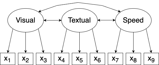
Figure 10.1: Path diagram for the Holzinger and Swineford model.
In some cases, the error terms \(\delta_1\) are included in the path diagram. We omit them here and in other path diagrams, but we always implicitly assume that observable variables have error terms associated with them.
To run a CFA using lavaan, we must first specify the model equations in a format that lavaan recognises. This is similar to, but different from, how regression formulas are specified, e.g., in lm. To say that the variables x1, x2, and x3 are associated with a latent variable called Visual, we write "Visual =~ x1 + x2 + x3". Note that the latent variable is on the left-hand side, even though it is the explanatory variable in our regression equations. Also note that we use =~ to indicate association between latent and observable variables.
In our example, we write the association between the latent and observable variables involved in a single string, with linebreaks:
We can then use the cfa function to fit the model and summary to view the results:
In order to estimate the coefficients \(\lambda_{1,1}, \ldots, \lambda_{9,3}\), we need to set the scale of \(\xi_1\), \(\xi_2\), and \(\xi_3\) in some way. The default method in lavaan is to use the so-called marker variable method, in which one \(\lambda_{i,j}\) is fixed to 1 for each \(\xi_j\). This is why the estimated \(\lambda_{i,j}\) is 1 for the first observed variable associated with each latent variable in the output for the fitted model:
Latent Variables:
                   Estimate  Std.Err  z-value  P(>|z|)
  Visual =~
    x1                1.000
    x2                0.554    0.100    5.554    0.000
    x3                0.729    0.109    6.685    0.000
  Textual =~
    x4                1.000
    x5                1.113    0.065   17.014    0.000
    x6                0.926    0.055   16.703    0.000
  Speed =~
    x7                1.000
    x8                1.180    0.165    7.152    0.000
    x9                1.082    0.151    7.155    0.000
The p-values in the rightmost column are for tests of the null hypothesis that \(\lambda_{i,j}=0\), i.e., that there is no association between \(x_i\) and \(\xi_j\).
The downside to using the marker variable method is that it makes it impossible to test hypotheses about the fixed \(\lambda_{i,j}\) (which is why the p-value column in the output is empty for these coefficients). Another common approach is therefore to instead fix the variance of the latent variables to 1, allowing the factor loading of all variables to vary. To use this approach, we add std.lv = TRUE to cfa:
10.2.2 Plotting path diagrams
To plot the path diagram of a factor model, we can use the semPaths function from the semPlot package.
We install the package and plot the path diagram for our model:
You’ll note that there are doubled-arrowed arrows pointing from the latent variables to themselves, and likewise for the observed variables. These are used to denote variances (i.e., the error terms \(\delta_i\) in the case of observed variables). To remove them, we can add exoVar = FALSE (for the latent variables) and residuals = FALSE (for the observed variables):
Fixed parameters are marked using dashed lines. To draw them as filled lines instead, add fixedStyle = 1:
10.2.3 Assessing model fit
An important part of CFA is evaluating how well the model fits the data. We can obtain additional measures of goodness-of-fit by adding fit.measures = TRUE when we run summary for our model:
Some commonly used measures of goodness-of-fit are:
- Chi-squared (\(\chi^2\)) test (
Model Test User Model): measures the difference between the covariance structure specified by the model and the empirical covariance structure. A low p-value indicates that these differ, i.e., that the model fails to capture the actual dependence structure. This was traditionally used in CFA but suffers from problems. For small sample sizes, the \(\chi^2\) test is sensitive to normality of the \(\delta_i\) and can have low power. For large sample sizes, it will in contrast virtually always yield a low p-value (because even if your model is close to the truth, it is probably not exactly true). For this reason, many practitioners now avoid using the \(\chi^2\) test. - Comparative Fit Index (CFI): ranges from 0 to 1, with values close to 1 being better. A value of at least 0.9 is seen as an indicator of a good fit.
- Tucker-Lewis Index (TLI): also known as the non-normed fit index (NNFI), (usually) ranges from 0 to 1, with values close to 1 being better. A value of at least 0.95 is seen as an indicator of a good fit.
- Root Mean Square Error of Approximation (RMSEA): ranges from 0 to 1, with values close to 0 being better. A value below 0.06 is seen as an indicator of a good fit.
- Standardized Root Mean Square Residual (SRMR): ranges from 0 to 1, with values close to 0 being better. A value below 0.08 is seen as an indicator of a good fit.
The rules of thumb for when these measures indicate a good fit are taken from Hu & Bentler (1999).
For our model, the CFI is 0.931 and the SRMR 0.065, indicating a good fit, while a TLI of 0.896 and an RMSEA of 0.092 indicate some problems with the fit. The results are inconclusive. This is fairly common for factor analysis models when the sample size ranges in the hundreds, as it does here. Larger sample sizes tend to lead to more stable results.
\[\sim\]
Exercise 10.3 Consider the attitude data that we studied in Section 10.1. Assume that theory stipulates that there are two underlying latent variables associated with the observed variables. The first, “career opportunity”, is hypothesised to be associated with advance, learning, and raises. The second, “employee treatment”, is associated with complaints, rating, raises, learning, and privileges. Neither latent variable is associated with critical.
Evaluate this hypothesised dependence structure by checking whether a confirmatory factor analysis yields a good fit. Plot the associated path diagram.
10.3 Structural equation modelling
Structural equation modelling (SEM), can be viewed as an extension of confirmatory factor analysis, in which we also model causal relationships between latent variables. This allows us to test relationships between different abstract concepts.
In a SEM, we distinguish between two types of latent variables:
- Endogenous variables: latent variables that are (partially) determined or explained by other latent variables in the model. The unexplained part is represented by an error term. Usually denoted \(\eta\).
- Exogenous variables: latent variables that are not determined or explained by the other latent variables in the model. Usually denoted \(\xi\) (in line with the notation we used for CFA).
10.3.1 Fitting a SEM
Let’s look at an example. We’ll use the PoliticalDemocracy dataset from lavaan, known from the classic SEM textbook by Bollen (1989):
The dataset concerns industrialisation and democracy in 75 developing countries in the 1960s. From subject-matter theory, there are three latent variables:
- Industrialisation in 1960 \(\xi_1\): associated with \(x_1\), \(x_2\), and \(x_3\),
- Democracy in 1960 \(\eta_1\): affected by \(\xi_1\) and associated with \(y_1\), \(y_2\), \(y_3\), and \(y_4\),
- Democracy in 1965 \(\eta_2\): affected by \(\xi_1\) and \(\eta_1\), and associated with \(y_5\), \(y_6\), \(y_7\), and \(y_8\).
\(\xi_1\) is exogenous, whereas \(\eta_1\) and \(\eta_2\) are endogenous. The theory is that industrialisation drives democracy in developing countries, i.e., that there is a causal relationship.
In addition to the above, it is believed that some of the observed variables are correlated, for instance \(y_1\) (expert ratings of the freedom of the press in 1960) and \(y_5\) (expert ratings of the freedom of the press in 1965). The model is summarised in Figure 10.2.
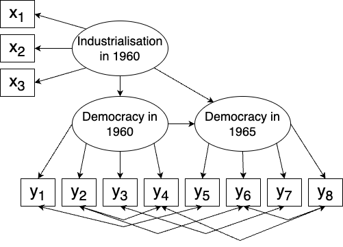
Figure 10.2: Structural equation model for the industrialisation and democracy model.
To specify the model for use with lavaan, we must specify three things. First, measurements models that describe the hypothesised relationships between latent variables and observed variables. These are written in the same way as for CFA, e.g., "Ind1960 =~ x1 + x2 + x3". Next, we need to specify latent variable regressions, describing relations between exogeneous and endogenous variables. These are written like regression formulas, e.g., "Dem1965 ~ Ind1960 + Dem1960". Finally, we specify the hypothesised correlations between observed variables, written with double tilde symbols: "y1 ~~ y5". The whole model then becomes:
model <- "
  # Measurement model:
  Ind1960 =~ x1 + x2 + x3
  Dem1960 =~ y1 + y2 + y3 + y4
  Dem1965 =~ y5 + y6 + y7 + y8

  # Latent variable regressions:
  Dem1960 ~ Ind1960
  Dem1965 ~ Ind1960 + Dem1960

  # Residual correlations:
  y1 ~~ y5
  y2 ~~ y4
  y2 ~~ y6
  y3 ~~ y7
  y4 ~~ y8
  y6 ~~ y8"
To fit the SEM specified above, we use sem:
The associations between the latent variables and the observed variables are all significant, as is the association between industrialisation in 1960 and 1965. The relations between the latent variables are also significant. However, some of the stipulated correlations between observed variables are not.
The output is very similar to that from cfa. In fact, cfa is a wrapper-function for sem, and the two have many arguments in common. We could for instance add std.lv = TRUE to the sem call to fix the variances of the latent variables.
Note that this changes not only the estimated coefficients, but also the p-values! The associations between the latent variables and the observed variables are still significant, as is the association between industrialisation in 1960 and 1965. The relations between democracy in 1965 and the other latent variables are however not significant.
The results from the hypotheses tests in a SEM can change if we change what parameters we keep fixed. This is unlikely to happen for large sample sizes, but when we have a complex model and a small sample size, as in this example, it is not uncommon. We should consider it a sign that our sample size is too small to test this model.
The p-values presented in the table are based on a normality assumption. If we like, we can use the bootstrap to compute p-values instead. To run the model again using the bootstrap with 1,000 bootstrap replicates to compute p-values, we do the following (which may take a minute to run):
10.3.2 Assessing and plotting the model
Model fit is assessed using the same measures as for CFA (see Section 10.2.3):
In this case, the \(\chi^2\) test and the CFI, TLI, RMSEA, and SRMR measures all indicate that the model is a good fit.
Just as for CFA, we can use semPaths to plot the path diagram for the model:
\[\sim\]
Exercise 10.4 Consider the HolzingerSwineford1939 data that we studied in Section 10.2. Assume that theory stipulates that there is an additional exogenous latent variable, “Mental maturity”, measured by the observed variables ageyr and sex, that causes the endogenous variables “visual”, “textual”, and “speed”.
Evaluate this hypothesised dependence structure by running a SEM. Plot the associated path diagram.
(Click here to go to the solution.)
Exercise 10.5 Download the treegrowth.csv dataset from the book’s web page. It contains simulated data inspired by Liu et al. (2016): five soil measurements, \(x_1, \ldots, x_5\), and four measurements of tree growth, \(y_1, \ldots, y_5\). It is hypothesised that the soil measurements relate to a latent variable describing environmental conditions, which affects a latent variable describing plant traits. The latter is associated with the tree growth measurements.
Evaluate this hypothesised dependence structure by running a SEM. Plot the associated path diagram.
10.4 Mediation and moderation in regression models
For hundreds of years, scurvy was the bane of many a sailor, killing at least two million between the 16th and 19th century (Drymon, 2008). In one of the first-ever controlled clinical trials, the Scottish physician James Lind showed that scurvy could be treated and prevented by eating citrus fruit.
But what was the mechanism involved in this?
In some cases, there is causal relationship between an explanatory variable and a response variable, but not a direct causal relationship. Instead, the explanatory variable affects a third variable, which in turn has an effect on the response variable.
Citrus and scurvy is an example of this. Eating citrus does not directly prevent scurvy, but it will raise your vitamin C levels, which in turn prevents scurvy. In this case, we say that vitamin C level is a mediator variable that mediates the effect of citrus-eating on scurvy.
An explanatory variable can have a direct effect (which does not act through the mediator) on the response variable, an indirect effect (which acts through the mediator), or both. The sum of the direct effect and the indirect effect is called the total effect of the explanatory variable. The purpose of dividing the total effect into these two parts is to understand the mechanism behind a known causal relationship, e.g., to understand how eating citrus prevents scurvy.
Mediation analysis is concerned with finding if a third variable (e.g., vitamin C levels) is involved in the mechanism through which a variable affects another. There should always be strong theoretical support for choosing a particular mediator variable; the analysis is used to confirm the theory, not to generate it. In addition to this, the following assumptions must be met:
- Correctly specified model: the functional relationships between the variables are correct and don’t interact with each other.
- Independent and homoscedastic errors: the error terms should not be correlated with each other or the explanatory variables and should all have the same variance.
- No omitted variables: the model accounts for all variables influencing the response variable. This is almost never true in practice – all models are wrong, but some are useful, as the saying goes54. For a mediation model to be useful, it is important that the effects of the omitted variables are negligible. In the case of vitamin C and scurvy, for instance, vitamin C uptake is affected by certain medical conditions, and if an effect like this is large enough and the conditions common enough, leaving it out from the model can skew the results substantially.
10.4.1 Fitting a mediation model
There are several packages that can be used for mediation analyses in R. We’ll use lavaan and the SEM framework – the formula language of which can also be used when all variables in the model have been observed. Our examples will use the following dataset from the psych package:
The data comes from an experiment in which people’s reactions to a news story were measured, along with their presumptions about the influence of the media, under two experimental conditions. The effect of the experimental condition is thought to be mediated by the presumed media influence. We visualise this using a diagram, as in Figure 10.3.
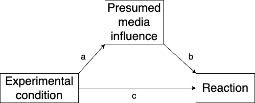
Figure 10.3: Mediation model for the news story reaction model.
Let \(x\) denote the experimental condition, \(m\) denote the presumed media influence, and \(y\) denote the reaction. Our mediation model is then as follows:
\[ m = a\cdot x + \epsilon_1\] \[y = b\cdot m + c\cdot x + \epsilon_2\] The direct effect of \(x\) is \(c\), the indirect effect is \(a\cdot b\), and the total effect is \(a\cdot b + c\).
First, we specify the model in a string. Then, we fit the model using sem, computing p-values using the bootstrap, and print the results using summary:
library(lavaan)
model <- "# Model:
          pmi ~ a*cond
          reaction ~ b*pmi + c*cond

          # Indirect and total effects:
          indirect_effect := a*b
          total_effect := indirect_effect + c"
m <- sem(model,
         data = Tal_Or,
         se = "bootstrap",
         bootstrap = 1000)
summary(m)
The most interesting part of the output is the first and last tables, showing estimates and p-values for the indirect and total effects (the output below has been cropped):
Regressions:
                   Estimate  Std.Err  z-value  P(>|z|)
  pmi ~
    cond       (a)    0.477    0.237    2.010    0.044
  reaction ~
    pmi        (b)    0.506    0.078    6.471    0.000
    cond       (c)    0.254    0.260    0.977    0.329

Defined Parameters:
                   Estimate  Std.Err  z-value  P(>|z|)
    indirect_effect   0.241    0.133    1.816    0.069
    total_effect      0.496    0.268    1.853    0.064
Changing from experimental condition 0 to 1 increases the presumed media influence by 0.477 units. This effect is significant (\(p=0.044\) in my run). A one unit increase in presumed media influence increases the reaction score by 0.506 units (also significant, \(p<0.001\)). However, the indirect effect of the experimental condition is not significant (\(p=0.069\)). Neither is the direct effect (\(p=0.329\)) or the total effect (\(0.064\)). In conclusion, there is no statistical evidence of the experimental condition affecting the reaction score, neither directly nor indirectly.
\[\sim\]
Exercise 10.6 Download the treegrowth.csv dataset from the book’s web page. The variable \(x_1\) describes calcium levels in soil, while \(x_4\) contains pH measurements. It is thought that the effect of \(x_1\) on plant height \(y_1\) is mediated by \(x_4\). Test this hypothesis.
10.4.2 Mediation with confounders
In mediation analysis, confounders are variables that potentially affect the mediator variable, the outcome, or both. Ignoring such variables can bias the estimates. In our example with presumed media influence, two potential confounders are gender and age. Adding them to our diagram, we get Figure 10.4.
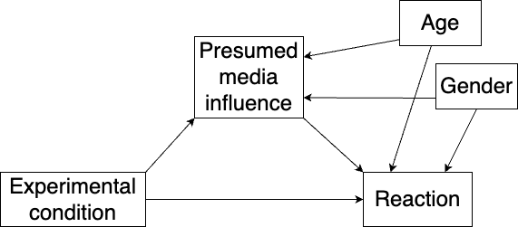
Figure 10.4: Mediation model with two confounders.
Letting \(x_1\) denote the experimental condition, \(x_2\) denote gender and \(x_3\) denote age, our model is now:
\[ m = a_1\cdot x_1 + a_2\cdot x_2 +a_3\cdot x_3 + \epsilon_1\] \[y = b\cdot m + c_1\cdot x + c_2\cdot x_2 + c_3\cdot x_3 + \epsilon_2\] The direct effect of \(x_1\) is \(c_1\), the indirect effect is \(a_1\cdot b\), and the total effect is \(a_1\cdot b + c\). All three effects are now adjusted for gender and age. We fit the model as follows:
10.4.3 Moderation
Mediation models often also include moderation effects. A moderator is a variable that modifies the strength of the relationship between two other variables, by strengthening, weakening, or even reversing the dependence. A visual representation of moderation is shown in Figure 10.5.
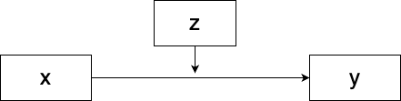
Figure 10.5: Model with moderation.
If \(x\) is an explanatory variable, \(z\) is a moderator, and \(y\) is the response variable, then a linear model including a moderation effect would look like this:
\[y=\beta_0+\beta_1 x+\beta_2 z+\beta_{12} xz.\]
You probably already know how to run a moderation analysis, even if the term “moderation” is unfamiliar to you. The effect of a moderator variable is namely described by the interaction term \(\beta_{12}\), just as in Sections 8.1.3 and 8.2.2. If \(\beta_{12}\) is significantly non-zero, then the moderation effect is significant. If \(\beta_1\) and \(\beta_{12}\) have the same sign, \(z\) strengthens the dependence between \(x\) and \(y\). If they have opposite signs, \(z\) weakens the dependence (and, if \(|\beta_{12}|>|\beta_{1}|\), reverses it).
If both variables are numeric, it is recommended to centre them; see Section 8.2.2 for more on this.
10.4.4 Mediated moderation and moderated mediation
Mediated moderation occurs when there is moderation of both the total and indirect effects of the explanatory variable. Returning to our example with presumed media influence, we’ll consider a model where a moderator variable, age, affects the paths from the explanatory variable, as shown in Figure 10.6:
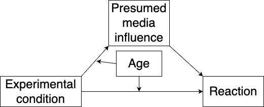
Figure 10.6: Model with mediated moderation.
model <- "# Model:
          pmi ~ a1*cond + a2*age + a12*cond:age
          reaction ~ b*pmi + c1*cond + c2*age + c13*cond:age

          # Moderated effects:
          mediated_moderation := a12*b
          total_moderated_effect := mediated_moderation + c13"
m <- sem(model,
         data = Tal_Or,
         se = "bootstrap",
         bootstrap = 1000)
summary(m)
Here, neither the mediated moderation nor the total moderated effect is significant.
Moderated mediation occurs when a moderator affects either the effect \(a\) of the explanatory variable on the mediator, or the effect \(b\) of the mediator on the response variable. Note that this is different from a model with confounders: confounders add new coefficients to the models, whereas a moderator adds an interaction term affecting \(a\) and/or \(b\).
Let’s say that we want to test whether age moderates the effect of the mediator on the response variable, as illustrated in Figure 10.7:
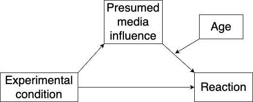
Figure 10.7: Model with moderated mediation.
To test this, we add age and an interaction between the moderator and age to the regression formula. First, we centre both variables, as they are numeric.
Without pipes:
With pipes:
library(dplyr)
Tal_Or |> mutate(pmi = scale(pmi, scale = FALSE),
                 age = scale(age, scale = FALSE)) -> Tal_Or
Next, we fit the model:
model <- "# Model:
          pmi ~ a1*cond
          reaction ~ b*pmi + c1*cond + c2*age + bc*pmi:age

          # Moderated effect:
          moderated_mediation := a1*bc"
m <- sem(model,
         data = Tal_Or,
         se = "bootstrap",
         bootstrap = 1000)
summary(m)
In this example, the moderated mediation effect is not significant.
\[\sim\]
Exercise 10.7 Download the treegrowth.csv dataset from the book’s web page. The variable \(x_1\) describes calcium levels in soil, \(x_2\) describes nitrate levels, and \(x_4\) contains pH measurements. It is thought that the effect of \(x_1\) on plant height \(y_1\) is mediated by \(x_4\), and that \(x_2\) moderates the relations between \(x_1\) and \(x_4\), and \(x_1\) and \(y_1\). Test this hypothesis of mediated moderation.
This aphorism is usually attributed to George Box, one of the greats of applied statistics. His 2013 memoir An Accidental Statistician is a must-read for those interested in the history of statistics.↩︎