9 Survival analysis and censored data
Survival analysis, or time-to-event analysis, often involves censored data. Censoring also occurs in measurements with detection limits, often found in biomarker data and environmental data. This chapter is concerned with methods for analysing such data.
After reading this chapter, you will be able to use R to:
- Visualise survival data,
- Fit survival analysis models, and
- Analyse data with left-censored observations.
9.1 The basics of survival analysis
Many studies are concerned with the time until an event happens: time until a machine fails, time until a patient diagnosed with a disease dies, and so on. In this section we will consider some methods for survival analysis (also known as reliability analysis in engineering and duration analysis in economics), which is used for analysing such data. The main difficulty here is that studies often end before all participants have had events, meaning that some observations are right-censored – for these observations, we don’t know when the event happened, but only that it happened after the end of the study.
The survival package contains a number of useful methods for survival analysis. Let’s install it:
We will study the lung cancer data in lung:
The survival times of the patients consist of two parts: time (time from diagnosis until either death or the end of the study) and status (1 if the observation is censored, 2 if the patient died before the end of the study). To combine these so that they can be used in a survival analysis, we must create a Surv object:
Here, a + sign after a value indicates right-censoring.
9.1.1 Visualising survival
Survival times are best visualised using Kaplan-Meier curves that show the proportion of surviving patients. Let’s compare the survival times of women and men. We first fit a survival model using survfit, and then draw the Kaplan-Meier curve using ggsurvplot from survminer:
install.packages("survminer")
library(survival)
library(survminer)
# Fit a survival model:
m <- survfit(Surv(time, status) ~ sex, data = lung)

# Draw the Kaplan-Meier curves:
ggsurvplot(m)
The plot shows the proportion of patients alive at different time points, starting at 100% at time 0. Tick marks along the lines show when censoring has occurred.
The average survival time is typically quantified using the median. Simply computing the median of the survival times is not a good idea, as this doesn’t take censoring into account. We can, however, get a reliable estimate of the median survival time for each group in our dataset from the Kaplan-Meier curves. The estimates are computed as the time at which the curves show that 50% of the patients have died.
To print the values for the survival curves at different time points, we can use summary. This way, we can get measures such as the one-year survival:
# Survival at all time points:
summary(m)

# One- and two-year survival (365.25 days and 730.5 days, respectively):
summary(m, times = c(365.25, 730.5))
We can customise the Kaplan-Meier plot, e.g., by adding confidence intervals to the estimates, adding a table showing the number at risk (number of patients at risk at different timepoints), and highlighting the median survival in each group:
ggsurvplot(m,
           conf.int = TRUE, # Add confidence intervals,
           risk.table = TRUE, # Show number at risk
           surv.median.line = "hv" # Show median survival
           )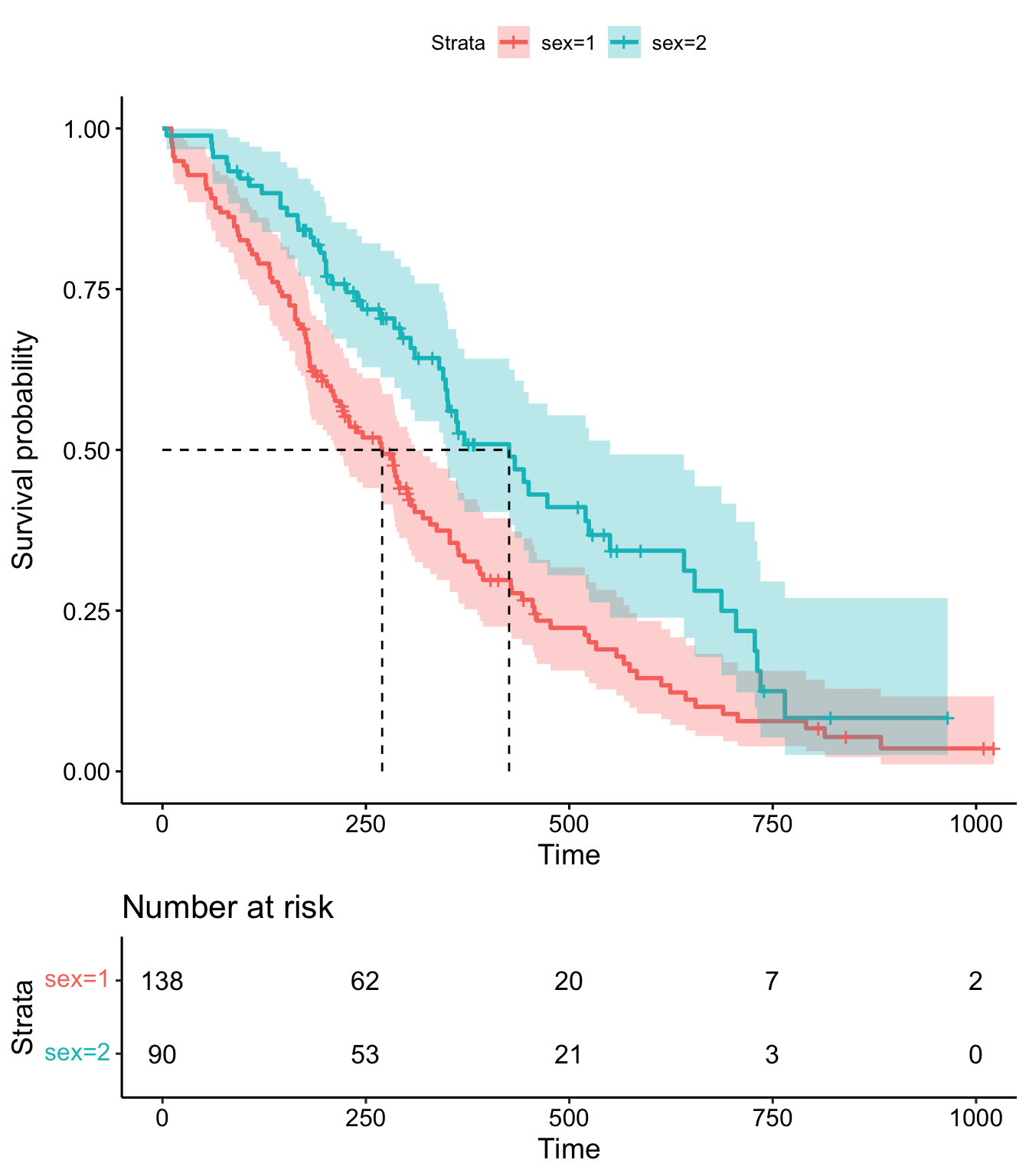
Figure 9.1: Kaplan-Meier plot for the lung data.
The resulting plot is shown in Figure 9.1. See ?ggsurvplot for more options and examples.
9.1.2 Testing for group differences
To test whether the survival curves of two groups differ, we can use the logrank test (also known as the Mantel-Cox or Mantel-Haenszel test), given by survdiff:
Another option is the Peto-Peto test, which puts more weight on early events (deaths, in the case of the lung data), and therefore is suitable when such events are of greater interest. In contrast, the logrank test puts equal weights on all events regardless of when they occur. The Peto-Peto test is obtained by adding the argument rho = 1:
If we wish to compare more than two groups, we can use a two-step procedure similar to ANOVA (Section 8.1.8). In the lung data, the ph.ecog variable is a measure of the patients’ well-being (where lower values are better). It divides the patients into four groups: 0, 1, 2, and 3. To test whether at least one of these groups differs from the others, we do a four-sample version of the logrank test:
The p-value is low (\(7\cdot 10^{-5}=0.00007\)) and we reject the null hypothesis that the survival curves are the same in all four groups. Next, we can test the pairwise differences using pairwise_survdiff from survminer:
There is no difference between groups 0 and 1 or between groups 2 and 3, but the differences between all other pairs of groups are significant. By default, the p-values presented in the table are adjusted for multiplicity using the Benjamini-Hochberg method (Section 3.7). You can control what method is used for the adjustment using the argument p.adjust.method; see ?pairwise_survdiff for details.
In addition to tests, we’re also interested in confidence intervals. The Hmisc package contains a function for obtaining confidence intervals based on the Kaplan-Meier estimator, called bootkm. This allows us to get confidence intervals for the quantiles (including the median) of the survival distribution for different groups, as well as for differences between the quantiles of different groups. First, let’s install it:
We can now use bootkm to compute bootstrap confidence intervals for survival times based on the lung data. We’ll compute an interval for the median survival time for females, and one for the difference in median survival time between females and males:
library(Hmisc)

# Create a survival object:
survobj <- Surv(lung$time, lung$status)

# Get bootstrap replicates of the median survival time for
# the two groups:
median_surv_time_female <- bootkm(survobj[lung$sex == 2],
                                  q = 0.5, B = 999)
median_surv_time_male <- bootkm(survobj[lung$sex == 1],
                                q = 0.5, B = 999)

# 95% bootstrap confidence interval for the median survival time
# for females:
quantile(median_surv_time_female,
         c(.025,.975), na.rm=TRUE)

# 95% bootstrap confidence interval for the difference in median
# survival time:
quantile(median_surv_time_female - median_surv_time_male,
         c(.025,.975), na.rm=TRUE)
To obtain confidence intervals for other quantiles, we simply change the argument q in bootkm.
\[\sim\]
Exercise 9.1 Consider the ovarian data from the survival package.
- Plot Kaplan-Meier curves comparing the two treatment groups.
- What are the median survival times in the two groups? Why do we get a strange estimate for the group where
rxis 2? - Compute a bootstrap confidence interval for the difference in the 90% quantile for the survival time for the two groups.
9.1.3 Hazard functions
The hazard function describes the rate of events at time \(t\) if a subject has survived until time \(t\). The higher the hazard, the greater the probability of an event. Hazard rates play an integral part in survival analysis, particularly in regression models.
Using ggsurvplot, we can plot the cumulative hazard function, estimated from the Kaplan-Meier survival curve, which shows the total hazard, or total amount of risk that has been accumulated, up until each timepoint:
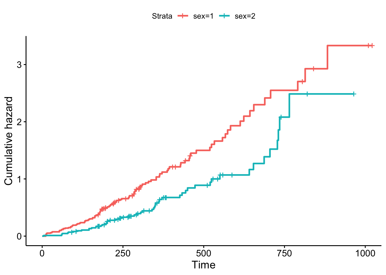
Figure 9.2: Cumulative hazards for the lung data.
The resulting plot is shown in Figure 9.2.
9.2 Regression models
In regression models for survival data, the response variable is a survival time. Using these models, we can study the effect of different variables on survival and predict survival.
9.2.1 The Cox proportional hazards model
The most commonly used regression model for survival data is the Cox proportional hazards model (Cox, 1972), fitted using coxph:
The exponentiated coefficients show the hazard ratios, i.e., the relative increases (values greater than 1) or decreases (values below 1) of the hazard rate when a covariate is increased one step, while all others are kept fixed:
In this case, the hazard increases with age (multiply the hazard by 1.017 for each additional year that the person has lived), and is lower for women (sex=2) than for men (sex=1).
As before, we can get a publication-ready table using tbl_regression:
The censboot_summary function from boot.pval provides a table of estimates, bootstrap confidence intervals, and bootstrap p-values for the model coefficients. The coef argument can be used to specify whether to print confidence intervals for the coefficients or for the exponentiated coefficients (i.e., hazard ratios):
# censboot_summary requires us to use model = TRUE
# when fitting our regression model:
m <- coxph(Surv(time, status) ~ age + sex,
           data = lung, model = TRUE)

library(boot.pval)
# Original coefficients:
censboot_summary(m, coef = "raw")

# Exponentiated coefficients:
censboot_summary(m, coef = "exp")

# Export to Word:
library(flextable)
censboot_summary(m, coef = "exp") |>
  summary_to_flextable() |>
  save_as_docx(path = "my_table.docx")
As the name implies, the Cox proportional hazards model relies on the assumption of proportional hazards, which essentially means that the effect of the explanatory variables is constant over time. In the case of sex in our lung example, it states that the hazard ratio between the sexes is constant over time, i.e., that there is no interaction between sex and time.
The proportional hazards assumption can be assessed visually by plotting the model residuals, using cox.zph and the ggcoxzph function from the survminer package. Specifically, we will plot the scaled Schoenfeld (1982) residuals, which measure the difference between the observed covariates and the expected covariates given the risk at the time of an event. If the proportional hazards assumption holds, then there should be no trend over time for these residuals. Use the trend line to aid the eye:
library(survminer)

ggcoxzph(cox.zph(m), var = 1) # age
ggcoxzph(cox.zph(m), var = 2) # sex

# Formal p-values for a test of proportional
# hazards, for each variable:
cox.zph(m)
In this case, there are no apparent trends over time (which is in line with the corresponding formal hypothesis tests), indicating that the proportional hazards model could be applicable here.
\[\sim\]
Exercise 9.2 Consider the ovarian data from the survival package.
- Use a Cox proportional hazards regression to test whether there is a difference between the two treatment groups, adjusted for age.
- Compute bootstrap confidence interval for the hazard ratio of age.
9.2.2 Repeated observation and frailty models
In some cases, we have repeated observations on the same individuals. An example can be found in the retinopathy data from the survival package:
In this dataset, there are two observations for each patient, because each patient has two eyes. If we ignore this information, we ignore the correlations between observations from the same patient, which can cause standard errors and p-values to become misleading.
There are two main approaches to dealing with repeated measurements in Cox models. The first approach is to use robust standard errors that take the correlations into account. For the retinopathy data, this can be achieved by adding cluster = id to the call to coxph. The second approach is to use a simple mixed model, called a frailty model, in which each individual has a unique excess risk (or “frailty”). To run such a model, we add + frailty(id) to the model formula. You’ll get to try both approaches in the following two exercises.
\[\sim\]
Exercise 9.3 Consider the retinopathy data from the survival package. In this dataset, there are multiple observations for each patient, and like in a mixed model, we need to take this into account when computing standard errors and p-values. id is used to identify patients and type, trt, and age are the explanatory variables we are interested in. Fit a Cox proportional hazards regression model, adding cluster = id to the call to coxph to include the information that observations from the same individuals are correlated. Is the assumption of proportional hazards fulfilled?
(Click here to go to the solution.)
Exercise 9.4 Repeat the analysis in the previous exercise, but use a frailty model instead. Does the conclusion change?
9.2.3 Accelerated failure time models
In many cases, the proportional hazards assumption does not hold. In such cases we can turn to accelerated failure time models (Wei, 1992), or AFT models for short. These are regression models that don’t rely on the assumption of proportional hazards. In AFT models, the effect of covariates is to accelerate or decelerate the life course of a subject.
While the proportional hazards model is semiparametric, accelerated failure time models are typically fully parametric, and thus involve stronger assumptions about an underlying distribution. In this case, we have to make assumptions about the distribution of the survival times.
Two common choices are the Weibull distribution and the log-logistic distribution. The Weibull distribution is commonly used in engineering, e.g., in reliability studies. The hazard function of a Weibull model is always monotonic, i.e., either always increasing or always decreasing. In contrast, the log-logistic distribution allows the hazard function to be non-monotonic, making it more flexible, and often more appropriate for medical studies. The distribution curves of these models are shown in Figure 9.3.
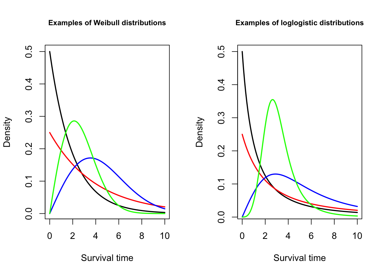
Figure 9.3: Distributions used for accelerated failure time models.
Let’s fit both types of models to the lung data and have a look at the results:
# Fit Weibull model:
m_w <- survreg(Surv(time, status) ~ age + sex, data = lung,
               dist = "weibull", model = TRUE)
m_w

# Fit log-logistic model:
m_ll <- survreg(Surv(time, status) ~ age + sex, data = lung,
                dist = "loglogistic", model = TRUE)
m_ll
Interpreting the coefficients of accelerated failure time models is easier than interpreting coefficients from proportional hazards models. The exponentiated coefficients show the relative increase or decrease in the expected survival times when a covariate is increased one step, while all others are kept fixed:
In this case, according to the log-logistic model, the expected survival time decreases by 1.4% (i.e., multiply by \(0.986\)) for each additional year that the patient has lived. The expected survival time for females (sex=2) is 61.2% higher than for males (multiply by \(1.612\)). This also means that the median survival time is 61.2% higher.
To obtain bootstrap confidence intervals and p-values for the effects, we follow the same procedure as for the Cox model, using censboot_summary. Here is an example for the log-logistic accelerated failure time model:
library(boot.pval)
# Original coefficients:
censboot_summary(m_ll, coef = "raw")
# Exponentiated coefficients:
censboot_summary(m_ll, coef = "exp")
\[\sim\]
Exercise 9.5 Consider the ovarian data from the survival package. Fit a log-logistic accelerated failure time model to the data, using all available explanatory variables. What is the estimated difference in survival times between the two treatment groups?
9.3 Competing risks
Survival studies often involve competing and mutually exclusive events that can occur. An example is found in the Melanoma data from the MASS package, where patients can die either from melanoma (one type of event) or die from other causes (another type of event):
This situation is commonly referred to as competing risks. In this section, we’ll see how we can visualise and analyse competing risks. First, we need to recode the status variable in the Melanoma data, which uses a non-standard coding that won’t work with the functions we will use. We also add some labels while we’re at it.
The coding we want to use for competing risks data is that 0 represents censoring (patient is alive), 1 represents the event of main interest (patient died of melanoma) and 2 represents the competing event (patient died from other causes).
Without pipes:
library(dplyr)
Melanoma$status <- factor(recode(Melanoma$status, "2" = 0, "1" = 1, "3" = 2),
                         labels = c("Alive",
                                    "Died from melanoma",
                                    "Died from other causes"))
Melanoma$sex <- factor(Melanoma$sex, levels = c(0, 1), labels = c("Female", "Male"))
With pipes:
library(dplyr)
Melanoma |>
  mutate(status = factor(recode(status, "2" = 0, "1" = 1, "3" = 2),
         labels = c("Alive", "Died from melanoma", "Died from other causes")),
         sex = factor(sex, levels = c(0, 1), labels = c("Female", "Male"))
         ) -> Melanoma
Next, let’s install two packages that we’ll need for the analysis:
Data with competing risks is sometimes analysed using a cause-specific approach, where each event type is analysed separately. Survival times for patients that have had other types of events are then censored by the other event. This allows us to study each type of event, but a major caveat is that the censoring due to other events needs to be independent from the rate of the type of event that we are studying in order for the analysis to be valid. That is, if we study death from melanoma, patients that are censored due to the end of the study need to have the same death rate from melanoma as patients who die from other causes. A different way of saying this is to say that the competing events need to be independent, which is a fairly strong assumption. If we are willing to make this assumption, we can draw Kaplan-Meier curves and fit regression models separately for each type of event, analysing them one by one.
A different approach uses the cumulative incidence function (CIF) which estimates the marginal probability for each type of event without assuming independence. In R, we can compute the CIF using cuminc, and then plot it using ggcuminc:
# Compute the CIF:
library(tidycmprsk)
m <- cuminc(Surv(time, status) ~ 1, data = Melanoma)

# Plot the CIF:
library(ggsurvfit)
ggcuminc(m, outcome = c("Died from melanoma", "Died from other causes"))
We can also compute the CIF stratified by some factor. For instance, we can compare the cumulative incidences for males and females (Figure 9.4):
cuminc(Surv(time, status) ~ sex, data = Melanoma) |>
  ggcuminc(outcome = c("Died from melanoma", "Died from other causes"))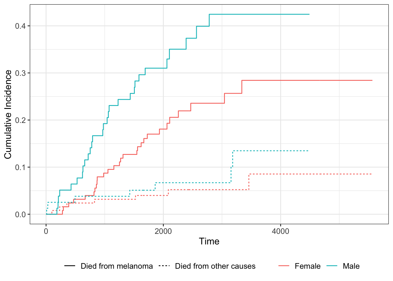
Figure 9.4: Cumulative incidence functions for the Melanoma data.
If we wish to model how the CIF is affected by explanatory variables, we can use the Fine-Gray regression model (Fine & Gray, 1999), which is an analogue to the Cox proportional hazards model based on the CIF. It is available through the crr function from the tidycmprsk package. The failcode argument specifies which event we are interested in modelling the CIF for:
# CIF for death from melanoma (status = 1):
m1 <- crr(Surv(time, status) ~ sex + age + ulcer,
         failcode = "Died from melanoma",
         data = Melanoma)
m1
# The presence of an ulcer increases the incidence.

# CIF for death from other causes (status = 2):
m2 <- crr(Surv(time, status) ~ sex + age + ulcer,
         failcode = "Died from other causes",
         data = Melanoma)
m2
# Age increases the incidence.
The coefficients are interpreted as in a Cox proportional hazards model, meaning it is useful to look at the exponentiated coefficients to get the hazard ratios:
As per usual, a publication-ready table can be obtained using tbl_regression:
9.4 Recurrent events
Another common type of survival data concerns recurrent events. A classic example of such data is the bladder2 dataset in the survival package, which describes recurrences of bladder cancer in 178 patients. Let’s have a look at it:
Note that there are two times associated with each event: a start time (start) and a stop time (stop). For patients with multiple events, e.g., the patient with id 5 that is listed on rows 5 and 6 in the data frame, the starting time for the second event is the stop time for the first event, and so on. We are interested in the difference between the two treatments shown in the rx variable.
For this kind of data, it is common that the time until a recurrence differs depending on how many previous recurrences an individual has had. In our example, the number of recurrences is listed in the enum variable. We can draw Kaplan-Meier curves grouped by the number of recurrences using the code below. Note that when we create the survival model, we need to specify both starting times and stop times in our Surv object.
m <- survfit(Surv(start, stop, event) ~ rx, data = bladder2)

# Draw the Kaplan-Meier curves, grouped by the enum variable:
ggsurvplot_group_by(m, bladder2, "enum") |>
  arrange_ggsurvplots(ncol = 2, nrow = 2)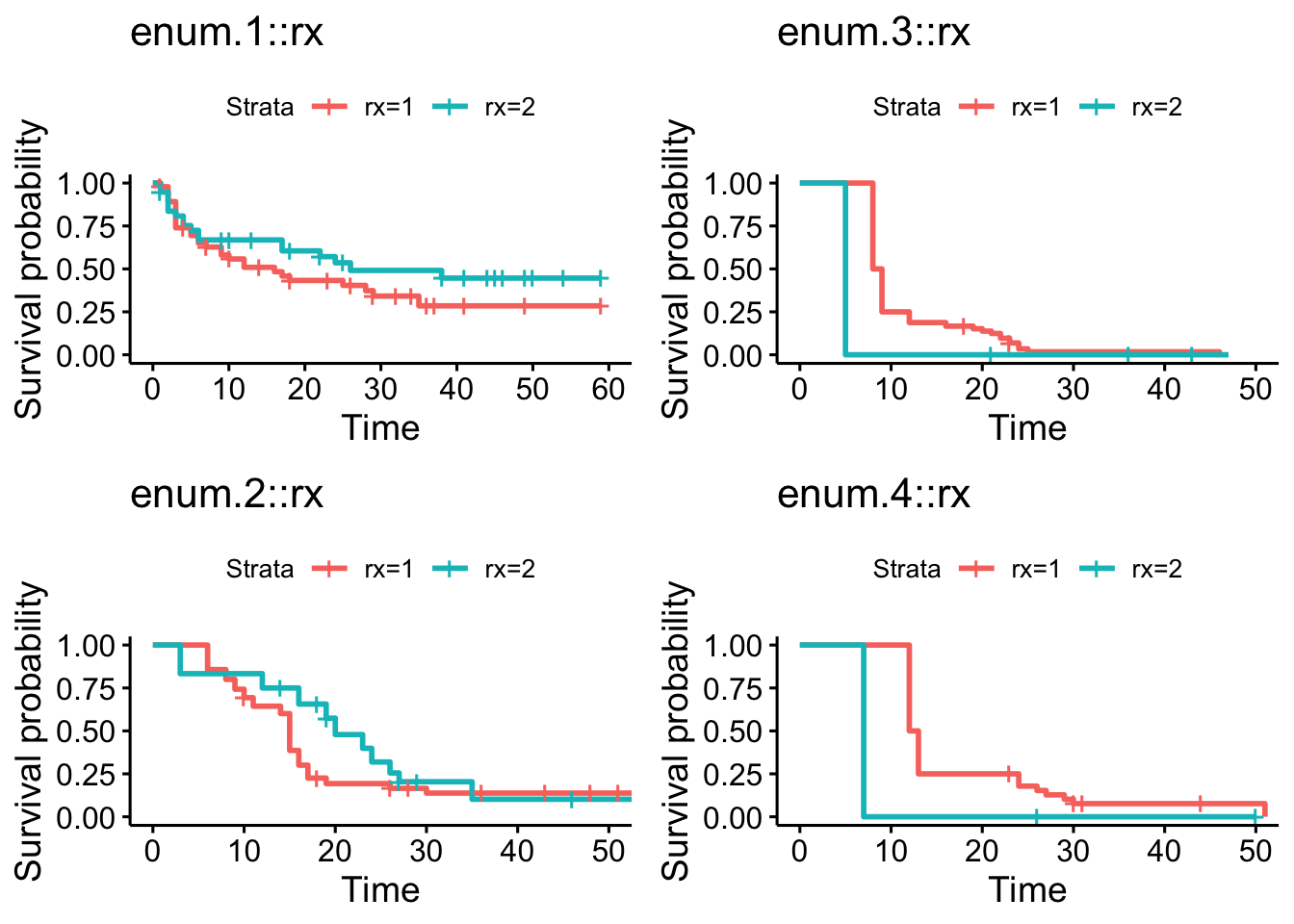
Figure 9.5: Kaplan-Meier curves grouped by the number of recurrences.
In this case, as seen in Figure 9.5, there are only a small number of patients with rx=2 that had three or four recurrences, making it difficult to compare the Kaplan-Meier curves to the right in the figure. We can, however, note that there appears to be a trend where the time to an event is shorter the more recurrences a patient has had. This could also be due to the fact that patients who for some reason have a shorter expected time between events tend to get more recurrences.
The Anderson-Gill model (Anderson & Gill, 1982) is an extension of the Cox proportional hazards model that handles recurrent events data. It is straightforward to fit this model using coxph:
The approach above is a little naïve, as it ignores the fact that we, like in Exercise 9.3, have repeated observations of the same patients. A better option would be to add cluster = id to indicate which observations belong to the same patient, or frailty(id) to run a frailty model:
# Model with robust standard errors:
m <- coxph(Surv(start, stop, event) ~ rx,
           cluster = id,
           data = bladder2)
summary(m)

# Frailty model:
m <- coxph(Surv(start, stop, event) ~ rx + frailty(id),
           data = bladder2)
summary(m)
An even better approach might be to stratify the model depending on the number of recurrences, which would allow us to model the fact that the time until an event seems to be lower for patients with multiple recurrences. This is called a Prentice-Williams-Peterson model (Prentice et al., 1981):
m <- coxph(Surv(start, stop, event) ~ rx + strata(enum),
           cluster = id,
           data = bladder2)
summary(m)

# A model with interactions between the treatment and the strata:
m <- coxph(Surv(start, stop, event) ~ rx * strata(enum),
           cluster = id,
           data = bladder2)
summary(m)
Regardless of which method we use, the treatment effect is not significant in this example. We obtain a publication-ready summary table using tbl_regression:
9.5 Advanced topics
9.5.1 Multivariate survival analysis
Some trials involve multiple time-to-event outcomes that need to be assessed simultaneously in a multivariate analysis. Examples include studies of the time until each of several correlated symptoms or comorbidities occur. This is analogous to the multivariate testing problem of Section 3.7.2, but with right-censored data. To test for group differences for a vector of right-censored outcomes, a multivariate version of the logrank test described in Persson et al. (2019) can be used. It is available through the MultSurvTests package:
As an example, we’ll use the diabetes dataset from MultSurvTest. It contains two time-to-event outcomes: time until blindness in a treated eye and in an untreated eye.
We’ll compare two groups that received two different treatments. The survival times (time until blindness) and censoring statuses of the two groups are put in a matrices called z and z.delta, which are used as input for the test function perm_mvlogrank:
# Survival times for the two groups:
x <- as.matrix(subset(diabetes, LASER==1)[,c(6,8)])
y <- as.matrix(subset(diabetes, LASER==2)[,c(6,8)])

# Censoring status for the two groups:
delta.x <- as.matrix(subset(diabetes, LASER==1)[,c(7,9)])
delta.y <- as.matrix(subset(diabetes, LASER==2)[,c(7,9)])

# Create the input for the test:
z <- rbind(x, y)
delta.z <- rbind(delta.x, delta.y)

# Run the test with 499 permutations:
perm_mvlogrank(B = 499, z, delta.z, n1 = nrow(x))
9.5.2 Bayesian survival analysis
At the time of this writing, the latest release of rstanarm does not contain functions for fitting survival analysis models. You can check whether this still is the case by running ?rstanarm::stan_surv in the Console. If you don’t find the documentation for the stan_surv function, you will have to install the development version of the package from GitHub (which contains such functions), using the following code:
# Check if the devtools package is installed, and start
# by installing it otherwise:
if (!require(devtools)) {
  install.packages("devtools")
}
library(devtools)
# Download and install the development version of the package:
install_github("stan-dev/rstanarm", build_vignettes = FALSE)
Now, let’s have a look at how to fit a Bayesian model to the lung data from survival:
library(survival)
library(rstanarm)

# Fit proportional hazards model using cubic M-splines (similar
# but not identical to the Cox model!):
m <- stan_surv(Surv(time, status) ~ age + sex, data = lung)
m
Fitting a survival model with a random effect works similarly and uses the same syntax as lme4. Here is an example with the retinopathy data:
9.5.3 Power estimates for the logrank test
The spower function in Hmisc can be used to compute the power of the univariate logrank test in different scenarios using simulation. The helper functions Weibull2, Lognorm2, and Gompertz2 can be used to define Weibull, lognormal, and Gomperts distributions to sample from, using survival probabilities at different time points rather than the traditional parameters of those distributions. We’ll look at an example involving the Weibull distribution here. Additional examples can be found in the function’s documentation (?spower).
Let’s simulate the power of a three-year follow-up study with two arms (i.e., two groups, control and intervention). First, we define a Weibull distribution for (compliant) control patients. Let’s say that their one-year survival is 0.9 and their three-year survival is 0.6. To define a Weibull distribution that corresponds to these numbers, we use Weibull2 as follows:
We’ll assume that the treatment has no effect for the first six months, and that it then has a constant effect, leading to a hazard ratio of 0.75 (so the hazard ratio is 1 if the time in years is less than or equal to 0.5, and 0.75 otherwise). Moreover, we’ll assume that there is a constant drop-out rate, such that 20% of the patients can be expected to drop out during the three years. Finally, there is no drop-in. We define a function to simulate survival times under these conditions:
# In the functions used to define the hazard ratio, drop-out
# and drop-in, t denotes time in years:
sim_func <- Quantile2(weib_dist,
      hratio = function(t) { ifelse(t <= 0.5, 1, 0.75) },
      dropout = function(t) { 0.2*t/3 },
      dropin = function(t) { 0 })
Next, we define a function for the censoring distribution, which is assumed to be the same for both groups. Let’s say that each follow-up is done at a random time point between 2 and 3 years. We’ll therefore use a uniform distribution on the interval \((2,3)\) for the censoring distribution:
Finally, we define two helper functions required by spower and then run the simulation study. The output is the simulated power using the settings that we’ve just created.
# Define helper functions:
rcontrol <- function(n) { sim_func(n, "control") }
rinterv  <- function(n) { sim_func(n, "intervention") }

# Simulate power when both groups have sample size 300:
spower(rcontrol, rinterv, rcens, nc = 300, ni = 300,
       test = logrank, nsim = 999)

# Simulate power when both groups have sample size 450:
spower(rcontrol, rinterv, rcens, nc = 450, ni = 450,
       test = logrank, nsim = 999)

# Simulate power when the control group has size 100
# and the intervention group has size 300:
spower(rcontrol, rinterv, rcens, nc = 100, ni = 300,
       test = logrank, nsim = 999)
9.6 Left-censored data and nondetects
Survival data is typically right-censored. Left-censored data, on the other hand, is common in medical research (e.g., in biomarker studies) and environmental chemistry (e.g., measurements of chemicals in water), where some measurements fall below the laboratory’s detection limits (or limit of detection, LoD). Such data also occur in studies in economics. A measurement below the detection limit, a nondetect, is still more informative than having no measurement at all – we may not know the exact value, but we know that the measurement is below a given threshold.
In principle, all methods that are applicable to survival analysis can also be used for left-censored data (although the interpretation of coefficients and parameters may differ), but in practice the distributions of lab measurements and economic variables often differ from those that typically describe survival times. In this section we’ll look at methods tailored to the kind of left-censored data that appears in applications in the aforementioned fields.
9.6.1 Estimation
The EnvStats package contains a number of functions that can be used to compute descriptive statistics and estimating parameters of distributions from data with nondetects. Let’s install it:
Estimates of the mean and standard deviation of a normal distribution that take the censoring into account in the right way can be obtained with enormCensored, which allows us to use several different estimators (details surrounding the available estimators can be found using ?enormCensored). Analogous functions are available for other distributions, for instance elnormAltCensored for the lognormal distribution, egammaCensored for the gamma distribution, and epoisCensored for the Poisson distribution.
To illustrate the use of enormCensored, we will generate data from a normal distribution. We know the true mean and standard deviation of the distribution and can compute the estimates for the generated sample. We will then pretend that there is a detection limit for this data, and artificially left-censor about 20% of it. This allows us to compare the estimates for the full sample and the censored sample, to see how the censoring affects the estimates. Try running the code below a few times:
# Generate 50 observations from a N(10, 9)-distribution:
x <- rnorm(50, 10, 3)

# Estimate the mean and standard deviation:
mean_full <- mean(x)
sd_full <- sd(x)

# Censor all observations below the "detection limit" 8
# and replace their values by 8:
censored <- x<8
x[censored] <- 8

# The proportion of censored observations is:
mean(censored)

# Estimate the mean and standard deviation in a naïve
# manner, using the ordinary estimators with all
# nondetects replaced by 8:
mean_cens_naive <- mean(x)
sd_cens_naive <- sd(x)

# Estimate the mean and standard deviation using
# different estimators that take the censoring
# into account:

library(EnvStats)
# Maximum likelihood estimate:
estimates_mle <- enormCensored(x, censored,
                               method = "mle")
# Biased-corrected maximum likelihood estimate:
estimates_bcmle <- enormCensored(x, censored,
                               method = "bcmle")
# Regression on order statistics, ROS, estimate:
estimates_ros <- enormCensored(x, censored,
                               method = "ROS")

# Compare the different estimates:
mean_full; sd_full
mean_cens_naive; sd_cens_naive
estimates_mle$parameters
estimates_bcmle$parameters
estimates_ros$parameters
The naïve estimators tend to be biased for data with nondetects (sometimes very biased!). Your mileage may vary depending on, e.g., the sample size and the amount of censoring, but in general, the estimators that take censoring into account will fare much better.
After we have obtained estimates for the parameters of the normal distribution, we can plot the data against the fitted distribution to check the assumption of normality:
library(ggplot2)
# Compare to histogram, including a bar for nondetects:
ggplot(data.frame(x), aes(x)) +
      geom_histogram(colour = "black", aes(y = ..density..)) +
      geom_function(fun = dnorm, colour = "red", size = 2,
                 args = list(mean = estimates_mle$parameters[1],
                                sd = estimates_mle$parameters[2]))

# Compare to histogram, excluding nondetects:
x_noncens <- x[!censored]
ggplot(data.frame(x_noncens), aes(x_noncens)) +
      geom_histogram(colour = "black", aes(y = ..density..)) +
      geom_function(fun = dnorm, colour = "red", size = 2,
                 args = list(mean = estimates_mle$parameters[1],
                                sd = estimates_mle$parameters[2]))
To obtain percentile and BCa bootstrap confidence intervals for the mean, we can add the options ci = TRUE and ci.method = "bootstrap":
# Using 999 bootstrap replicates:
enormCensored(x, censored, method = "mle",
              ci = TRUE,  ci.method = "bootstrap",
              n.bootstraps = 999)$interval$limits
\[\sim\]
Exercise 9.6 Download the il2rb.csv data from the book’s web page. It contains measurements of the biomarker IL-2RB made in serum samples from two groups of patients. The values that are missing are in fact nondetects, with detection limit 0.25.
Under the assumption that the biomarker levels follow a lognormal distribution, compute bootstrap confidence intervals for the mean of the distribution for the control group. What proportion of the data is left-censored?
9.6.2 Tests of means
When testing the difference between two groups’ means, nonparametric tests like the Wilcoxon-Mann-Whitney test often perform very well for data with nondetects, unlike the t-test (Zhang et al., 2009). For data with a high degree of censoring (e.g., more than 50%), most tests perform poorly. For multivariate tests of mean vectors, the situation is the opposite, with Hotelling’s \(T^2\) (Section 3.7.2) being a much better option than nonparametric tests (Thulin, 2016).
\[\sim\]
Exercise 9.7 Return to the il2rb.csv data from Exercise 9.7. Test the hypothesis that there is no difference in location between the two groups.
9.6.3 Censored regression
Censored regression models can be used when the response variable is censored. A common model in economics is the Tobit regression model (Tobin, 1958), which is a linear regression model with normal errors, tailored to left-censored data. It can be fitted using survreg.
As an example, consider the EPA.92c.zinc.df dataset available in EnvStats. It contains measurements of zinc concentrations from five wells, made on eight samples from each well, half of which are nondetects. Let’s say that we are interested in comparing these five wells (so that the wells aren’t random effects). Let’s also assume that the eight samples were collected at different time points, and that we want to investigate whether the concentrations change over time. Such changes could be non-linear, so we’ll include the sample number as a factor. To fit a Tobit model to this data, we use survreg as follows.
library(EnvStats)
?EPA.92c.zinc.df

# Note that in Surv, in the vector describing censoring 0 means
# censoring and 1 no censoring. This is the opposite of the
# definition used in EPA.92c.zinc.df$Censored, so we use the !
# operator to change 0's to 1's and vice versa.
library(survival)
m <- survreg(Surv(Zinc, !Censored, type = "left") ~ Sample + Well,
             data = EPA.92c.zinc.df, dist = "gaussian")
summary(m)
Similarly, we can fit a model under the assumption of lognormality:
m <- survreg(Surv(Zinc, !Censored, type = "left") ~ Sample + Well,
             data = EPA.92c.zinc.df, dist = "lognormal")
summary(m)
Fitting regression models where the explanatory variables are censored is more challenging. For prediction, a good option is models based on decision trees, studied in Section 11.5. For testing whether there is a trend over time, tests based on Kendall’s correlation coefficient can be useful. EnvStats provides two functions for this: kendallTrendTest for testing a monotonic trend, and kendallSeasonalTrendTest for testing a monotonic trend within seasons.